1. Introduction
The desire for an accurate, high-resolution quantitative precipitation estimate transcends meteorological, hydrological, and agricultural needs. Unfortunately, it is unlikely that the obstacles presented by the current gauge and radar observing network will ever be surmounted to the point where such a product may be realized. This assertion is especially palpable over expanses of complex terrain where the utility of these data is severely limited. Moreover, the current gauge and radar network will never provide adequate coverage over large bodies of water.
The inadequacy of the current network has facilitated a search for alternative tools with which to remotely sense precipitation. The interest in a satellite-based platform lies in the assumption that this information can potentially provide a cost-effective source of data over temporal and spatial scales not possible from any other in-situ or remotely sensed observing system. These precipitation estimates would be a valuable commodity in many hydrological and meteorological applications where high-resolution estimates are not routinely available. The modeling community, for example, would embrace the opportunity to use rainfall rates to initialize surface hydrology schemes and provide estimates of latent heating over regions not covered by the current observing network.
Another such application is in heavy precipitation and flash flood forecasting. These data would serve to augment the primary observing network since the temporal and spatial coverage of satellite estimates exceeds those that are presently available to operational forecasters. Currently, even the best surface rainfall observing systems fail to capture the true spatial distribution exhibited by precipitating systems. It is known that hourly raingauge observations are limited by numerous coverage and availability problems (Fulton et al. 1998). In addition, the accuracy and reliability of these gauges is also an issue. Although radar estimates are superior to gauge reports in areal coverage and resolution, they suffer from limitations due to the assumptions and implementation of the standard Z-R power law relationship (e.g., Battan 1973, Doviak and Zrnic 1984). Moreover, both methods are severely limited over mountainous terrain and large bodies of water where coverage is poor or non-existent.
Although the first weather satellites were commissioned in the early 1960s, the practice of extracting rainfall rate information from satellite radiance data did not become operational until nearly 15 years later. During the middle 1970s, the Satellite Analysis Branch (SAB) of NESDIS began using a manual technique to obtain real-time precipitation estimates from the Geostationary Orbiting Earth Satellite number 5 (GOES-5) radiance data. This method involved graphically comparing the evolution of a precipitating weather system from sequential half-hourly infrared images to concurrent raingauge data. This information was used to predict the rainfall rates based upon updated imagery. As additional computer resources became available, this manual procedure was replaced by the semi-automated Interactive Flash Flood Analysis (IFFA) technique (Scofield and Oliver 1977, Scofield 1987), which is still in service today. National Weather Service (NWS) field offices and River Forecast Centers (RFCs) ultimately use these forecasts for flash flood guidance.
The primary objective of this research is to perform a systematic evaluation of the NESDIS Auto-Estimator (A-E), a satellite-based algorithm for the estimation of rainfall (Vincente et al. 1998). This effort is intended to serve as an independent benchmark for the assessment of A-E products, as well as to provide a measure of the reliability of satellite-based precipitation algorithms in general. It is important that the accuracy of the A-E be established, since this algorithm is currently being proposed by NESDIS as the successor to the operational IFFA technique used by SAB forecasters at the National Centers for Environmental Prediction (NCEP).
2. Precipitation Estimates and Analyses
a) NESDIS Auto-Estimator
Two versions of the A-E, hereafter referred to as "standard" and "demonstration", were evaluated in this study. Both versions were run in parallel from spring 1997 through January 1999 and remained unchanged for the purpose of evaluation. Specific details regarding the standard version of the algorithm are outlined in Vincente et al. (1998).
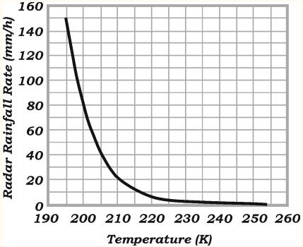
The fundamental algorithm employed by both versions of the A-E uses the GOES 10.7-mm channel to compute instantaneous rainfall rates every 30 min. These rates are determined from an empirically derived power-law regression curve between cloud-top temperature and radar-based rainfall estimates (Fig. 1). The instantaneous rain-rate estimates are adjusted based upon the cloud-top temperature gradient, growth rate, and vertically integrated moisture. Computation of these parameters requires two consecutive images as well as precipitable water and relative humidity fields from a recent Eta Model (Black 1994) forecast. Hourly rainfall rates are computed by taking a weighted average of instantaneous rainfall rates from 3 consecutive satellite images. One, 6-, and 24-h accumulations of precipitation are produced by summing up the individual hourly rainfall estimates.
The two versions of the A-E evaluated in this study differ in that the standard version is completely automated, while the demonstration algorithm incorporates an interactive component and an orographic correction. The interactive element of the demonstration A-E allows SAB forecasters to subjectively decrease the cloud-top temperatures for a particular weather system, enhancing the rain rate. This manual adjustment is especially useful during warm-top (stratiform) rain events, where observed precipitation rates are much greater than those obtained from the unadjusted regression curve (Fig. 1). During this evaluation, there no way SAB forecasters could manually increase the observed cloud-top temperatures, which would reduce rainfall rates.
Fig. 1 Mean rainfall rate for each temperature from 195 to 255 K computed from collocated pairs of radar-derived rainfall rate estimates and IR cloud-top temperature. Power-law fit between radar-derived rainfall estimates and cloud-top temperature (solid line). (Adapted from Vincente et al. 1998)
The orographic correction in the demonstration A-E is based upon the assumption that higher (lower) precipitation rates exist along the upslope (downslope) side of complex terrain. This adjustment factor is based upon the simple relationship,
![]() (1)
(1)
Here, Z is the terrain height and is the 850-mb wind from the most recent 6-h Eta model forecast. Precipitation estimates over 1- and 24-h periods were re-mapped from their native satellite projection to the national Hydrologic Rainfall Analysis Project (HRAP) grid at approximately a 4-km horizontal resolution.
b) Stage III Precipitation Estimates
The hourly NCEP Stage III precipitation analyses (Fulton et al. 1998) were used as the primary "ground truth" observation for the A-E verification. The Stage III analysis is an hourly, multi-sensor product developed at the NWS Office of Hydrology. This product is derived from the Stage II multi-sensor estimate, which uses a multivariate optimal estimation procedure (Seo 1998) to integrate 1-h gauge data into a WSR-88D rainfall analysis (Stage I). However, the Stage III has an advantage over the Stage II and Stage IV analyses, in that it undergoes a manual quality control during processing at the River Forecast Centers (Fig. 2). This interactive component of the data processing allows for the removal of erroneous precipitation such as areas contaminated by anomalous propagation.
In order to obtain the 24-h cumulative totals of observed precipitation from the Stage III data, consecutive 1-h analyses were summed over the period of interest. If a 1-h estimate was missing during a particular 24-h period, the 24-h estimate was omitted from the evaluation. Estimates over water were not used in the verification. This step was taken because these estimates are from radar only.
c) 24-h gauge-only precipitation estimates
The NCEP 24-h (daily) gauge-only precipitation analysis serves as a second data set used for verification of the A-E and data quality assurance for the Stage III product. The gauge-only analyses use the same optimal estimation theory as the Stage III analyses. This daily precipitation analysis is an improvement in resolution and coverage over the 1-h gauge data due to the greater number of observations (~6000) incorporated into the analysis, many of which report solely on a 24-h basis.
d) Radar-only Precipitation Estimates
Radar-only precipitation estimates (Stage I) were used for an intra-comparison between the various operational precipitation products. These radar-derived precipitation estimates are generated by applying the standard NWS Z-R relationships to WSR-88D reflectivities at the nearly 100 NWS radar sites. Individual radar estimates are then mosaiced onto the HRAP grid to form a national composite. A more complete discussion of the processing of these data is presented in Fulton et al. (1998).
3. Data Methods and Analysis
a) River Forecast Centers Used in the Verification
Most of the results presented in this study were derived from a comparison between the A-E and Stage III precipitation analyses evaluated over the Arkansas-Red Basin RFC (ABRFC) (Fig. 2). As stated above, the Stage III products were chosen as the basis for this evaluation because are considered to provide the best available analysis of rainfall over a RFC domain. However, due to the various sources of error that frequently accompany multi-sensor precipitation estimates, different levels of confidence were placed on the analyses with each of the RFCs. Additionally, not all RFCs routinely perform a quality control of the Stage III data. Therefore, only Stage III analyses from those RFCs that generally provide the highest quality estimates were used in this study. Consequently, the ABRFC was chosen as the primary RFC for this evaluation because it is believed to have one of the best representations of surface precipitation (Seo, personal communication).
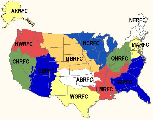
Fig. 2 Locations and areal coverage for the River Forecast Centers (RFCs) over the US. Those RFCs show are Alaska RFC (AKRFC), North West RFC (NWRFC), California-Nevada RFC (CNRFC), Colorado Basin RFC (CBRFC), Missouri Basin RFC (MBRFC), Arkansas-Red Basin RFC (ABRFC), Western Gulf RFC (WGRFC), Ohio RFC (OHRFC), Lower Mississippi RFC (LMRFC), Southeast RFC (SERFC), Northeast RFC (NERFC), and Mid-Atlantic RFC (MARFC).
b) Determination of valid grid boxes for verification
Statistics were calculated over aggregate resolutions of 1, 2, 4, 8, 16, 32, and 64 HRAP grid boxes (approximately 4-, 8-, 16-, 32-, 64-, 128-, and 256-km respectively) within a RFC domain. Because the HRAP grid is on a polar stereographic projection, the total area enclosed within a grid box varies with latitude. To eliminate the bias introduced by variable areal coverage, the mean precipitation within each grid box was normalized to the average amount of precipitation over a 4x4km area.
Data within collocated grid boxes of estimated and observed precipitation that contained either missing or questionable data were not included in the sample. A data sample includes all estimate and observation pairs within a RFC domain that satisfies the quality controls described below. As a result, not all grid boxes within the RFC were used. To be included in the sample, collocated boxes of both the precipitation estimate and analysis needed to contain a non-flagged, non-zero value. A grid box was flagged if the data were located over water, missing, or the result of satellite transmission problems. If one of the collocated grid boxes was flagged or both grid boxes contained zero precipitation (0/0), it was not included in the sample. Consequently, no 0/0 pairs were used in the evaluation. It was presumed that there was significant skill in predicting zero precipitation where there were no clouds. The purpose for removal of the zero precipitation pairs was to increase the critical assessment of the A-E evaluation. In order to be included in the statistical database for each combination of temporal and spatial scale, an aggregate sample within a RFC domain needed to contain more thn five valid data pairs.
Statistics for different thresholds of observed precipitation were also computed for the entire suite of spatial and temporal scales evaluated in this study. The thresholds were chosen for each temporal window as follows:
In order to be included in a statistical sample, the observed amount of precipitation needed to exceed the specified threshold. If the observed precipitation was less than the prescribed amount, the data were not included in the sample regardless of whether or not the estimated precipitation amount exceeded that threshold. The minimum amount of precipitation reported by the A-E is 2.0 mm independent of the precipitation estimate period.
During the computation of monthly means, statistics for the 1- and 24-h temporal resolutions were weighted according to the number of valid data pairs within an RFC domain during that period. This approach was taken so statistical scores from large-scale events consisting of thousands of valid grid boxes carried more weight than small-scale events consisting of only a few grid boxes.
Due to the large quantity of data generated through the comparisons over the various temporal and spatial scales, only a subset of the total volume of results will be discussed in this paper. Overall, the performance of the statistical measures employed in this study varied modestly across the suite of spatial resolutions. The skill scores improved slightly when evaluations were performed on a lower resolution grid, such as the 132x132-km domain, compared to the native (4x4-km) grid. However, these improvements were not significant enough to proclaim any one areal coverage superior to the others. Consequently, the results presented here demonstrate the findings from this study as a whole.
4. An intra-comparison between the precipitation analyses used in this study
Before the performance of the A-E could be evaluated, an intra-comparison between the various precipitation analyses employed in this study was performed. The purpose of this assessment was to establish the best benchmark with which to compare the scores from the A-E. It must be emphasized that a comparison between the various analyses suggests nothing about the accuracy of any one observing platform, due to the amount of uncertainty, or error, inherent in each of these products. Moreover, comparisons of the radar- or gauge-only estimates against the milti-sensor Stage III product are not independent. The purpose of this exercise is to obtain a measure of the disagreement between the various precipitation analyses, which can then be compared to the A-E scores.
Results from the 1- and 24-h, ~8x8-km (2x2 HRAP grid boxes) conditional analysis (precipitation observed within a grid box from both analyses) are presented. Comparisons using the 1-h radar-only dataset began in February 1998 and continued throughout the evaluation period. The 24-h gauge-only analyses were made available beginning in April 1998. Because complete ABRFC-wide coverage by the radar-only precipitation estimates was inconsistent, only the results from the conditional statistics (precipitation observed in both grid boxes) are discussed. Data from the 24-h, 76.20-mm and 1-h, 25.40-mm thresholds are not displayed because there were an insufficient number of samples to be provide meaningful statistics.
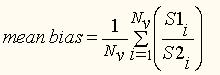
The monthly mean 24-h bias scores over ABRFC are presented in Figs. 3a and b. For this study, the mean bias was defined to be the ratio between the two precipitation analyses within a valid grid box,
 (1)
(1)
Here, Nv is the number of valid grid boxes within the ABRFC domain, S1 and S2 represent the observed amount of precipitation within a grid box from schemes 1 and 2 respectively.
Overall, there is very little spread in the scores among the thresholds in each of the intra-comparisons. The analyses that were most similar in terms of areal precipitation were the 24-h Stage III and gauge-only products (Fig 3a). Bias scores were near 1.00 from April though December for the 2.54-mm threshold indicating that the monthly mean 24-h precipitation amounts from these products were very similar. This is not totally unexpected since the Stage III estimates use the 1-h gauge observations to adjust the radar-derived amounts (Fulton et al. 1998); however, the 24-h gauge analysis does utilize many additional observations that report solely on a daily basis.
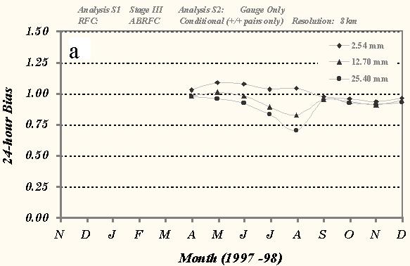
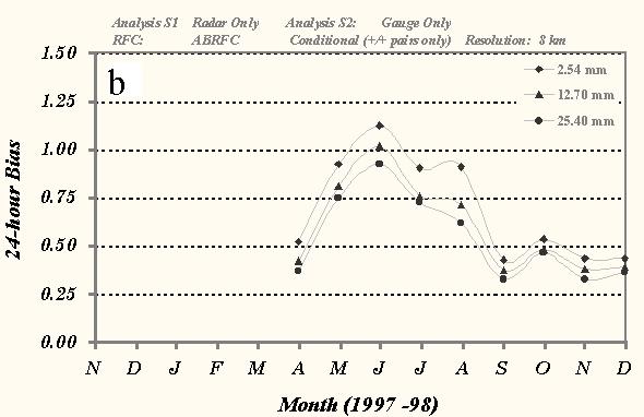
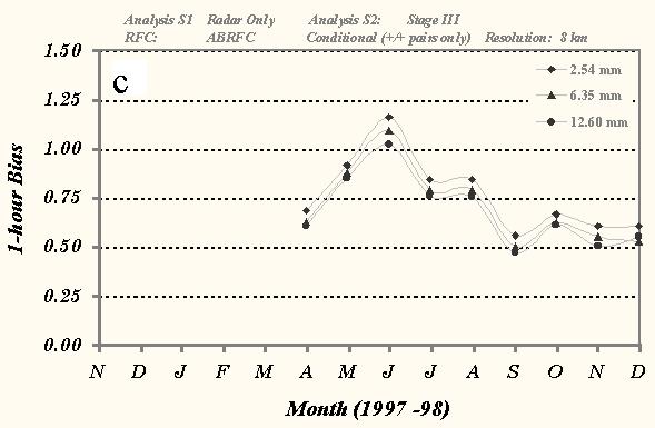
Fig. 3 Time series of monthly mean conditional bias scores between a) 24-h Gauge-only and Stage III analyses, b) 24-h Radar-only and Gauge only analyses, and c) 1-h Radar-only and Stage III analyses over ABRFC for various thresholds of precipitation. Only 8x8-km grid box precipitation amounts were used in the statistical sample.
Comparisons with the radar-only data (Figs. 3b and c) suggest a seasonal trend in the precipitation estimates at both the 24- and 1-h periods. Radar-estimated precipitation peaked during the warm months (May, June, July, and August) near 1.00 before declining to near 0.50 for the cool season. Range degradation is the likely cause for this underestimation of precipitation during the cool season, as the radar beam tends to overshoot the shallow, stratiform-type precipitating systems
The monthly mean 1- and 24-h correlation coefficient scores over ABRFC are presented in Fig. 4. In general, the results show that scores from the various precipitation analyses decrease uniformly with larger thresholds. The comparison between the gauge-only and Stage III analysis demonstrates the largest month-to-month volatility (Fig. 4a). Scores at the 2.54-mm threshold ranged averaged 0.72 over the entire evaluation. Results from the comparison between the gauge and radar-only analyses are lower than those from the Stage III product (Fig. 4b). The data do not indicate a seasonal trend as was evident in the bias scores and the mean correlation coefficient value over the 9-month period is 0.57. Coefficient scores for the 1-h radar and Stage III analyses do suggest a season trend in this statistical measure. The mean score over the evaluation was 0.59, very similar to than the 24-h gauge/radar results. However, the scores show a distinct decrease in mean value from the warm season (0.64) to the cool season (0.53).
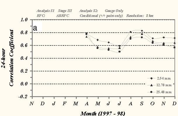
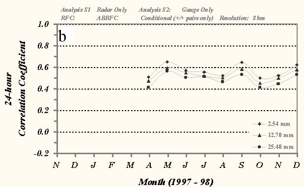
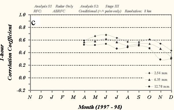
Fig. 4 As in Fig. 3 except for monthly mean correlation coefficient
5.0 An evaluation of the NESDIS Auto-Estimator
An evaluation of the standard version of the A-E over ABRFC during the period from November 1997 through December 1998 is presented in this section. Results from an assessment of the demonstration version were nearly identical to those of the standard, and thus, are not discussed here. However, a case study in which the skill of the demonstration and standard versions are compared is presented in section 6.
Some gauges of skill presented in this study are those traditionally computed from contingency table-based models. These measures include False Alarm Rate (FAR), Probability of Detection (POD) (Donaldson et al 1975), and Critical Success Index (CSI) (Doswell et al. 1990, Schaefer 1990). The CSI has also been referred to as the Threat Score (Bermowitz and Zurndorfer 1979, Junker et al. 1992) and is used widely in operational forecast verification (Doswell et al. 1990). The use of CSI as an appraisal of skill is appropriate for this validation due to the trivial nature of null (0/0) events.
Two non-table based skill measures, bias and correlation coefficient, were also selected for the evaluation of the A-E. Bias scores were computed from (1) with the satellite-base estimate and the Stage III analysis serving as S1 and S2 respectively. All non-table measures were computed from the conditional pool of A-E/Stage III precipitation pairs. The conditional results include all valid grid boxes within the RFC domain that contained both observed (Stage III) and forecasted (A-E) precipitation, with the observed amount exceeding a minimum threshold (section 3). The conditional statistics are particularly useful because they provide an appraisal of how the A-E performs when the algorithm correctly identifies the location of precipitation. Results from the unconditional precipitation data sample were nearly identical to those of the conditional pool and will not be discussed.
The A-E was originally developed to estimate precipitation from deep convective systems. Such systems are common during the late spring and summer over ABRFC. In contrast, large-scale non-convective precipitation events are more frequent across the region during the late fall and winter. Consequently, a comparison of the A-E skill between the cool and warm seasons is of interest. For this study, the warm season is defined to include the months of May through August, while the cool season includes the months from November to February.
5.1 Verification Results from the 24- and 1-h A-E
Figure 5 illustrates the ABRFC-wide monthly mean precipitation for both the Stage III and standard A-E during the evaluation period. Evident in the 24-h data at each threshold are high-amplitude monthly fluctuations in the A-E precipitation compared to the Stage III analysis (Fig. 5a). This modulation was also present in the unconditional results (not shown). The Stage III analysis did exhibit some month-to-month variability during the late summer, as precipitation amounts increased more than 50% between August and September. This increase in observed rainfall over ABRFC was due to a number of tropical systems that moved northward from the Gulf of Mexico. A case study of one of these systems (Tropical Storm Francis) is presented in section 6.
In nine of fourteen months during the study, the 24-h A-E underforecasted the amount of mean precipitation at the 2.54-mm threshold, primarily during the late fall and winter. From May through August, however, the A-E overestimated the mean precipitation. In addition, the difference between the monthly Stage III and A-E amounts grow larger with increasing threshold of observed precipitation. This trend toward larger disparities with increasing threshold suggests that the A-E did not correctly identify the cores of maximum observed precipitation.
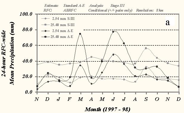
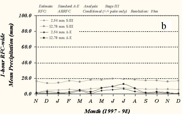
Fig. 5 Time series of monthly mean a) 24-h precipitation (mm) over ABRFC for the 2.54- and 25.40-mm thresholds of precipitation and b) 1-h precipitation (mm) over ABRFC for the 2.54- and 12.70-mm thresholds of precipitation for conditional grid box pairs from the standard version of the A-E and the Stage III precipitation analysis. The dark lines represent the A-E amounts while the gray-shaded lines depict the Stage III totals. Only 8x8-km grid box amounts were used in the statistical sample.
As in the 24-h, but to a lesser degree, the 1-h A-E precipitation amounts also fluctuate relative to the Stage III amounts throughout the evaluation (Fig. 5b). Overall, the A-E forecasted precipitation for the 2.54 and 12.70 mm thresholds fell below the observed amounts during this period. The mean 1-h precipitation from the A-E increased during the months of May through August, similar to the 24-h results. Following this increase in forecasted rainfall, the A-E appears to have had difficulty generating precipitation through the late fall and winter. A case study examining the performance of the A-E during a convective event in December 1998 is presented in section 6.
a) 24-h A-E skill measure results
Fluctuations similar to those exhibited by the 24-h mean precipitation fields are also evident in the table scores across each threshold (Fig. 6). As suggested by the monthly mean precipitation comparison, the skill of the 24-h A-E decreases with an increase in the minimum amount of observed precipitation. Mean POD scores over the entire 14-month evaluation period decrease from 0.51 to 0.41, while FARs increase from 0.26 to 0.45 for the 2.54- and 25.40-mm threshold amounts respectively. Mean CSIs decrease commensurably with the changes in POD and FARs, with values decreasing from 0.40 for the 2.54 mm threshold to 0.20 for the 25.40 mm threshold of observed precipitation.
An examination of the CSIs indicates that the A-E demonstrated better skill during the warm season compared to the cool season across each threshold of observed precipitation. For example, the mean CSI increased from 0.32 during the late fall and winter to 0.45 in the summer at the 2.54 mm level (Fig. 6a). The skill measure that showed the greatest improvement from cool to warm season was the POD. The mean value for the cool season was 0.37, which increased to 0.67 during the summer. However, the FARs also increased between these seasons, from 0.22 to 0.38. This increase in FAR was primarily due to a tendency of the A-E to spread out the precipitation estimates over a larger area than was observed in the warm season. This apparent predisposition is likely due to cold-cloud cirrus shields that frequently accompany deep convection. The cold cloud-top temperatures contaminate the A-E-derived precipitation by enhancing the forecasted precipitation over a larger area than is observed.
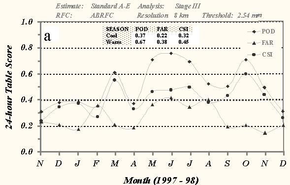
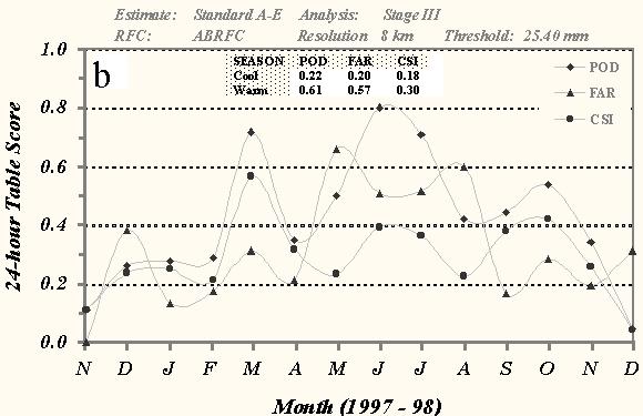
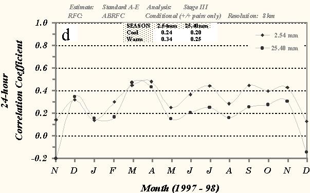
Fig. 6 Time series of monthly mean 24-h POD, FAR, and CSI over ABRFC for the a) 2.54- and b) 25.40-mm thresholds of observed precipitation, c) bias scores for the 2.54- and 25.40-mm thresholds, and d) correlation coefficient scores between the standard version of the A-E and the Stage III precipitation analysis for conditional grid box pairs. The dark lines represent the A-E amounts while the gray-shaded lines depict the Stage III totals. Only 8x8-km grid box amounts were used in the statistical sample. The table at the top of each graph depicts the seasonal averages for each measure.
Similar trends in the table scores can be seen across greater thresholds of observed precipitation with the skill of the A-E improving from the cool to the warm season (Fig. 6b). These measures also indicate a marked decrease in skill by the A-E as the threshold increases. Notice that POD scores fall off during the cool season, with a score 0.22 for the 25.40-mm threshold (Fig. 6b). The CSI for the larger threshold (0.18) is also much lower compared to the 2.54 mm score.
A strong sensitivity to the threshold of observed precipitation is seen in the FARs during the warm season (Fig. 6b). The FAR increases from 0.20, at 2.54 mm, to 0.62 for the 25.40 mm threshold, exceeding the POD score (0.61) during this period. Consequently, the CSI score for this period decreases to 0.30 for the larger threshold.
The 24-h monthly mean bias also exhibits strong monthly and seasonal variability (Fig. 6c). The bias scores generally decrease with larger thresholds of observed precipitation, although mean scores over the entire evaluation for the 2.54 and 25.40 mm thresholds were comparable at 1.15 and 0.92 respectively. The A-E significantly underforecasted the precipitation over ABRFC during the cool season with a mean bias for the 2.54 mm threshold of 0.61. However, fortunes were reversed during the warm season as the mean bias increased to 2.00, meaning the A-E overestimated the amount of rainfall by 2 fold.
The computed correlation coefficient scores for the 24-h A-E precipitation estimates are shown in Fig. 6d. This measure demonstrated the greatest monthly and seasonal consistency compared to the previously presented skill measures. Scores for the 2.54 mm threshold are 0.24 and 0.34 during the cool and warm seasons respectively, which are significantly less than the 0.60 value considered indicative of a moderate linear correlation. The 24-h mean coefficient scores ranged between 0.20 and 0.45 for much of the evaluation indicating that only 4 to 18% of the A-E/Stage III sample fit the statistical model.
a) 1-h A-E skill measure results
The skill of the A-E over short periods is of greater interest to operational flash flood forecasters since these events typically occur over 6 hours or less. Furthermore, a decision as too whether to issue a watch or warning is based upon rainfall data assimilated over much shorter periods. Thus, examining the 1-h skill scores may provide a measure of the utility of the A-E in providing guidance to forecasters for these events.
Similar to the 24-h results, the 1-h POD and CSI scores show that the skill of the A-E improves from the cool to the warm season across all thresholds of observed precipitation (Figs. 7). The mean 2.54 mm threshold CSI increased from 0.08 during the late fall and winter to 0.17 for the summer (Fig. 7a). POD also increased significantly from 0.12 to 0.43. Results for the 12.70 mm threshold show that the skill of the A-E decreased slightly compared to the 2.54 mm totals with mean CSI scores increased from 0.04 during the late fall and winter to 0.13 for the summer (Fig. 7b). Notice that the mean FARs for the 1-h A-E forecasts exceeded the POD scores for each month of this evaluation across both thresholds. These 1-h table measure scores are much lower than those exhibited by the 24-h precipitation estimates, indicating that the A-E has less skill over 1-h than the 24-h period.
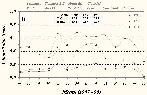
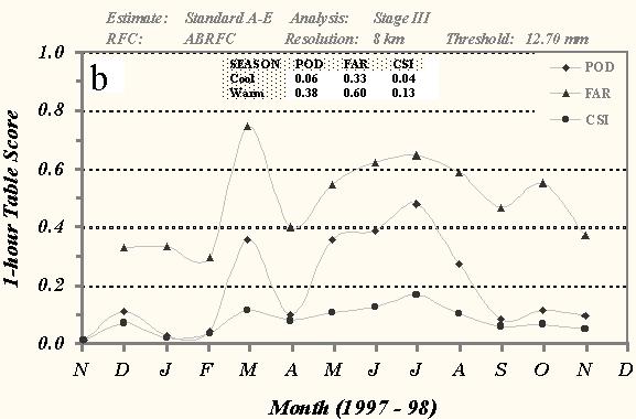
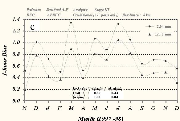
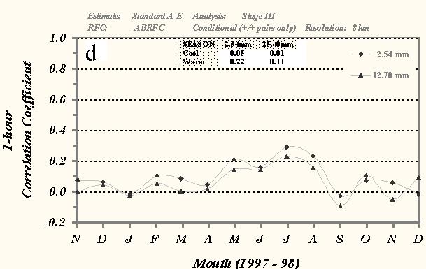
Fig. 7 Time series of monthly mean 1-h POD, FAR,
and CSI over ABRFC for the a) 2.54- and b) 12.70-mm thresholds of observed precipitation, c) bias scores for the
2.54- and 12.70-mm thresholds, and d) correlation coefficient scores between the standard version of the A-E and
the Stage III precipitation analysis for conditional grid box pairs. The dark lines represent the A-E amounts while
the gray-shaded lines depict the Stage III totals. Only 8x8-km grid box amounts were used in the statistical sample.
The Table at the top of each graph depicts the seasonal averages for each measure.
Monthly mean bias scores over the course of the evaluation are shown in Fig. 7c. These measures also exhibit the month-to-month volatility seen in the mean precipitation (Fig 5). Overall, bias scores decrease with increasing threshold. The mean 1-h bias over the entire evaluation for the 2.54 mm threshold was 0.82, indicating that the A-E underforecasted the amount of precipitation when compared to the Stage III analyzed amounts over ABRFC. The seasonal mean bias increased from 0.66 during the late fall and winter to 1.08 for the warm season.
The correlation coefficient between the 1-h A-E and Stage III products demonstrates less monthly variation compared to any of the previously presented 1-h measures (Fig. 7d). The scores suggest that the 1-h A-E generally possess little skill at these temporal resolutions. Calculated mean values for the 2.54 mm threshold were 0.05 during cool season, which increased to 0.22 for the warm season. Scores for the 12.70 mm threshold were below the zero line on four occasions (1/98, 3/98, 9/98, and 11/98), indicating a negative linear correlation.
5.2 Inter-period Variability of the A-E Precipitation Estimates
Thus far, the statistical measures computed in this study have been presented as monthly mean values over the course of the evaluation. Unfortunately, the computed monthly averages do not provide an indication of the variability in the statistics within a particular month. An estimate as to the predictability of the performance measures over short periods of time would serve to benefit users of the A-E, who are typically concerned with precipitation estimates over 24 hours or less, and want to know the reliability of these data from one estimate to the next.
To better illustrate the short-term variability of the A-E, the hourly correlation coefficients over ABRFC during a convectively active seven-day window in July 1998 are depicted in Fig. 8. This particular period was chosen because rainfall was observed within the RFC during all but 12 of the 1-h periods (168 possible). In addition, since the A-E was originally developed for use during warm season convective events, an evaluation during this time will provide an appraisal of the A-E under nearly ideal conditions.
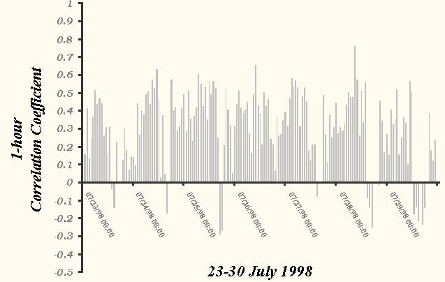
Fig. 8 Time series of hourly (UTC) unconditional correlation coefficient values between the Standard A-E and the Stage III analysis over ABRFC for the 2.54-mm threshold of observed (Stage III) precipitation between 0000 UTC 23 and 0000 UTC 30 July 1998.
The hourly correlation coefficient scores in Fig. 8 display a high degree of variability from one 1-h precipitation estimate to the next. Values range from below -0.300 on 25 July to above 0.700 on 28 July. A closer inspection of the daily trend indicates that the scores usually peaked above 0.500 just before 1200 UTC, while lowest values typically occurred around 1800 UTC.
In spite of the hour-to-hour volatility in the values, the similarity in timing of the daily maximums and minimums suggests a diurnal trend in the data. To investigate this possibility, the data were averaged according to the estimate hour over the seven-day period. The resulting 24-h time series strongly implies a diurnal trend in the correlation coefficient scores (Fig. 9). The largest mean scores, above 0.400, occur just after 0000 Local Daylight Time (LDT) and decrease to negative values around 1200 LDT (noon).
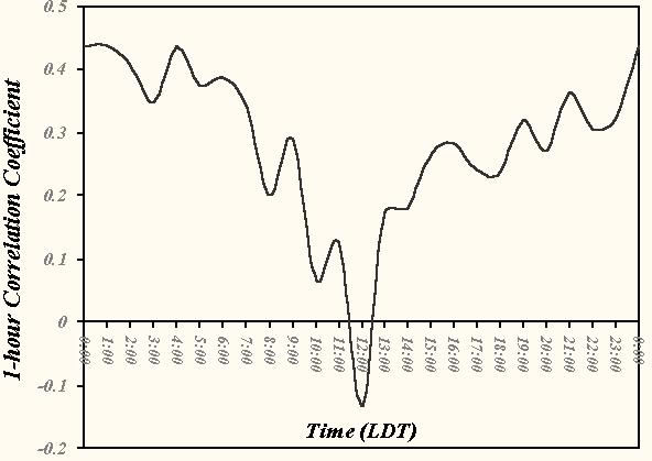
Fig. 9 Time series of mean hourly unconditional correlation coefficient values between the Standard A-E and the Stage III analysis over ABRFC for the 2.54-mm threshold of observed (Stage III) precipitation. Hourly averages were derived from the data depicted in Fig. 8 and converted to Local Daylight Time (LDT) for display.
The forcing for this diurnal trend is not immediately apparent. It is likely that the mean hourly precipitation over this period had a significant impact in the coefficient scores; however, the timing of the maximum and minimum do not coincide with that expected if the convection were forced by the solar cycle. To better compare the precipitation trend with the coefficient scores, a plot of the hourly mean precipitation for both the Stage III and standard A-E are depicted in Fig. 10. The data exhibit a similar diurnal trend, with the signal from the A-E much more amplified than that of the Stage III precipitation. The observed mean rainfall amounts are at a minimum around noon LDT (~4 mm) and increase into the evening, peaking at around 2200 LDT. The trend in the A-E rainfall is similar, although the minimum occurs about 1 hour after that of the Stage III data.
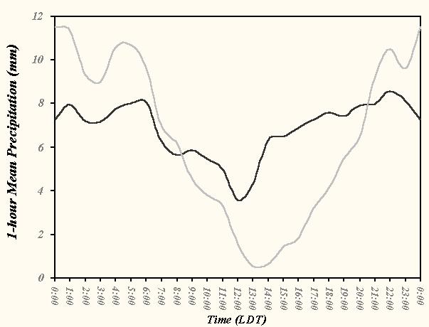
Fig. 10 Time series of hourly conditional mean
precipitation from the Standard A-E (gray-shaded line) and the Stage III analysis (black line) over ABRFC for the
2.54-mm threshold. Hourly averages were derived from the data depicted in Fig. 8 and converted to Local Daylight
Time (LDT) for display.
Most interesting is the ostensible predisposition for the A-E to overpredict the RFC-wide mean precipitation during the night and underpredict the rainfall during the day. Notice that the ratio of estimate-to-observed precipitation is near 1.0 at 8 AM and 8 PM (2200) LDT. It is not known whether the solar cycle has any impact in the GOES 10.7-mm radiance data used in the derivation of the rainfall estimates or if the algorithm is sensitive to changes in surface skin temperature over the cloud-free regions. It is more likely that the heavier precipitation is associated with deep convection and accompanying cirrus contamination, while the lighter amounts are produced by warm-top clouds.
6.0 Case Studies
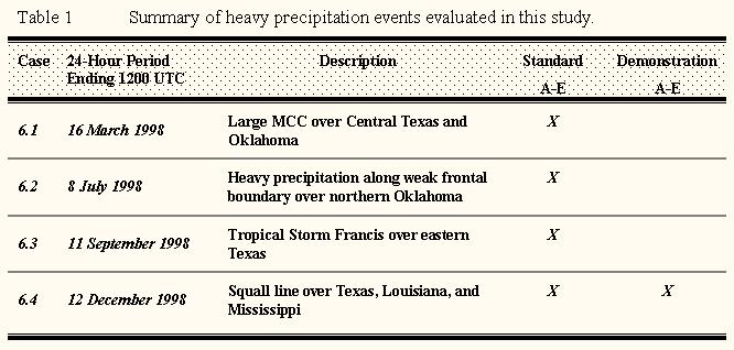
A number of heavy precipitation events were selected to test the skill of the A-E under a variety of meteorological conditions. Individual cases are presented based upon the type of phenomena responsible, the location of the precipitation, and the time of year. A summary of these events is provided in Table 1.0.
6.1 Texas and Oklahoma: 16 March 1998
This case examines the performance of the A-E with a large mesoscale convective complex that grew rapidly over northern Texas and Oklahoma between 15 and 16 March 1998. Extremely heavy rainfall and flash flooding characterized this event, with an expansive area of gauge-reported precipitation in excess of 76.20-mm (3.00 inches) extending from central Texas northward (Fig. 11a). Mean rainfall over ABRFC from the stage III analyses (Fig. 11b) totaled 25.40 mm for the 2.54-mm threshold of observed precipitation (Table 2).
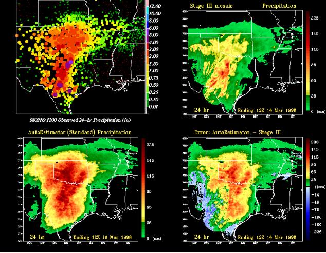
Fig. 11 The 24-hour precipitation estimates valid 12 UTC 16 March 1998 from a) individual 24-hour rain gauge reports (inches) categorized and color coded according to amount, b) a mosaic of RFC Stage III precipitation analyses (mm), and c) the Standard Auto-Estimator (mm). d) 24-hour precipitation error field (mm) derived from the difference between the Standard Auto-Estimator (c) and the Stage III analysis (b).
A comparison of the 24-h storm totals from the Stage III (Fig. 11b) precipitation against the standard A-E (Fig. 11c) shows that the A-E spread out the heaviest precipitation over a much larger area than was observed. Rainfall estimates from the satellite-based algorithm were in excess of 100 mm over much of central Oklahoma and central Texas. The wide areal coverage of both the A-E and Stage III rainfall within ABRFC provided a large number of forecast "hits" (precipitation predicted and observed within a grid box), leading to high POD scores at each threshold (Table 2).
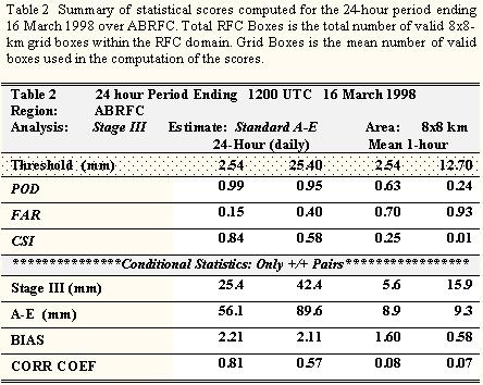
Note that the 24-h FAR increases from 0.15 to 0.40 between thresholds. The reduction in skill is also seen in a decrease of the CSI score from 0.84 to 0.58 for the 2.54 and 25.40 mm thresholds respectively. The poorer performance at larger thresholds is primarily due to the tendency of the A-E to extend the heaviest precipitation over a much larger area than was observed. The A-E overestimated the total amount of precipitation over a large area during this period (Fig 11d) as 24-h bias scores were in excess of 2.00 at each threshold.
Overall, the 1-h A-E amounts possess less skill than the 24-hour totals (Table 2). Mean observed amounts increase nearly 3 fold between the 2.54 and 12.70mm threshold, from 5.6 to 15.9 mm; however, the A-E precipitation over this same region did not appreciably increase (from 8.9 to 9.3 mm) This disparity suggests that the A-E had difficulty identifying the cores of maximum precipitation over the short periods in this case. This contention is further supported by the drop in mean CSI from 0.25, at the 2.54-mm threshold, to 0.01 at 12.70 mm. In addition, the correlation coefficient values did not exceed 0.10 for either threshold.
6.2 Stationary Front over Northern Oklahoma: 8 July 1998
Between 1200 UTC 7 and 1200 UTC 8 July 1998, moderate to heavy rainfall was observed along the Oklahoma and Kansas border. This precipitation was focused along a weak, quasi-stationary frontal zone that extended from New Mexico eastward into Kentucky. Gauge reports between 50.80 mm (2.00 inches) and 101.60 mm (4.00 inches) were common over this region (Fig. 12a). Mean rainfall over ABRFC from the stage III analyses (Fig. 12b) totaled 19.20 mm for the 2.54-mm threshold of observed precipitation (Table 3).
A comparison of the 24-h rainfall estimates from the A-E (Fig. 12c) and the error field (Fig. 12d) indicate that the algorithm overpredicted the amount and areal coverage of precipitation during this event. The satellite algorithm produced 72.2 mm of conditional rainfall at the 2.54-mm threshold over ABRFC. This was not just a case of excessive areal coverage by the satellite-based routine. The A-E precipitation exceeded 300 mm and errors were greater than 250 mm at some locations (Fig. 12d). The 24-h conditional bias scores indicate that the A-E overestimated the mean precipitation within the ABRFC by 376% and 282% for the 2.54- and 25.40-mm thresholds respectively.
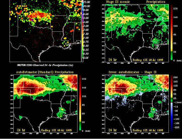
Fig. 12 As in Fig. 11 except for 12 UTC 8 July 1998
POD values for both thresholds (0.90 and 0.91) were largely the result of an overproduction of rainfall by the A-E. This tendency during convective events also led to an increase in the FARs from 0.15 to 0.40 between thresholds. Consequently, the CSI fell from 0.62 at 2.54-mm to 0.30 at 25.40-mm.
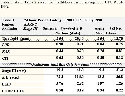
This event provided the best 1-h correlation coefficient scores of any case presented in this study, as values exceeded 0.20 for both thresholds. Table measures were similar for both threshold with POD scores near 0.70, FARs above 0.75, and CSI values below 0.20. Mean bias scores over the 24-h period were 1.97 at 2.54-mm and 1.26 at the 25.40 mm thresholds.
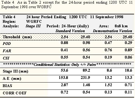
6.4 Tropical Storm Francis: September 11, 1998
This event coincided with the landfall of Tropical Storm Francis along the Texas Gulf Coast on 10 September 1998. Heavy precipitation was observed from east-central, Texas into western Louisiana, with the heaviest amounts located near the Texas coastline. Gauge amounts of more than 152.40 mm (6.00 inches) were common along the Texas Gulf Coast with a few reports greater than 203.20 mm (8.00 inches) (Figs. 13a).
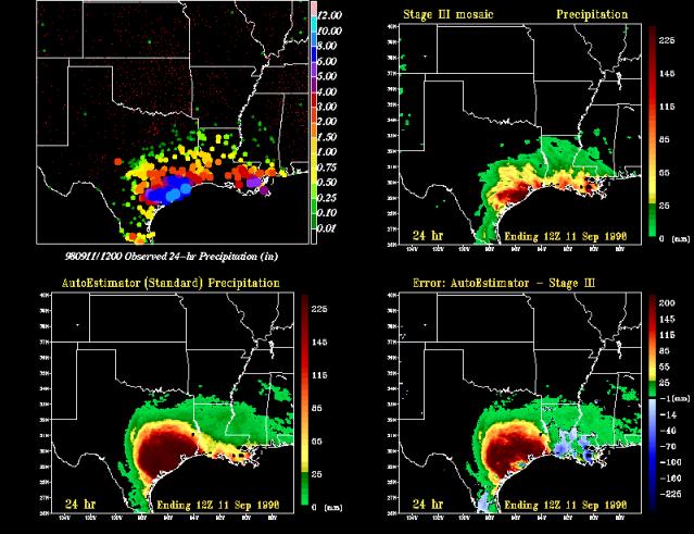
Fig. 13 As in Fig. 11 except for 12 UTC 8 July 1998
A comparison of the 24-h storm totals from the Stage III (Fig. 13b) precipitation against the satellite-based estimates (Fig. 13c) illustrates that the A-E again spread out the heaviest precipitation over a much larger area than was observed. Rainfall estimates from the standard A-E were in excess of 200 mm over much of east-central Texas. This over estimation of rainfall is manifested in the large bias scores of 2.87 and 1.48 for each threshold respectively.
6.5 Louisiana Squall Line: 12 December 1998
This case was selected to show how the A-E performed with late-season deep convection. As discussed earlier, the skill of the A-E is expected to improve for convective systems compared to those consisting of primarily warm-top, stratiform precipitation. The results presented in Section 5 indicated that the A-E had difficulty generating precipitation for events after September 1998. This case will provide some insight as to whether this systematic error was due to an under-representation of convective systems or a more fundamental problem with the algorithm. In addition, SAB forecasters utilized the rain-rate adjustment algorithm of the demonstration A-E to enhance the precipitation rates for this system. Thus, an examination of the impact from this manual correction is also presented.
During the 24-h period between 1200 UTC 11 and 1200 UTC 12 December 1998, a strong line of convection developed over the south central US. Gauge-based rainfall reports in excess of 101.60 mm (4.00 inches) were observed from eastern Texas into central Mississippi (Fig. 14a). Stage III 24-h amounts (Fig. 14b) also indicate a second rainfall maximum extending from north central Texas into Oklahoma. A comparison between the satellite-based algorithms (Fig. 14c) and the observed totals suggests that the A-E completely missed the location of heaviest rainfall.
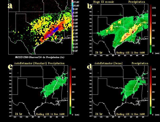
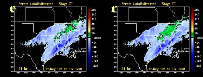
Fig. 14 The 24-hour precipitation estimates valid 12 UTC 12 December 1998 from a) individual 24-hour rain gauge reports (inches) categorized and color coded according to amount, b) a mosaic of RFC Stage III precipitation analyses (mm), c) the Standard Auto-Estimator (mm), and d) the Demonstration Auto-Estimator (mm). 24-hour precipitation error field (mm) derived from the difference between the A-E and the Stage III analysis and e) the Standard Auto-Estimator, f) the Demonstration Auto-Estimator.
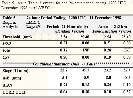
The 24-h precipitation estimates from the demonstration and standard versions of the A-E are presented in Figs. 14c and d. Very subtle differences exist between the these two versions as SAB forecasters modulated the rainfall rates only slightly during this event. Rainfall totals reveal an underestimation from both algorithms. Mean 24-h precipitation amounts at the 2.54-mm threshold from the standard version were 5.4 mm before the manual correction, which were then increased to 8.0 mm in the demonstration version at the lowest threshold (Table 5). Both of these amounts are much less than the ~23 mm that was observed. The overall skill demonstrated by the A-E in this event was the weakest of those cases presented in this study. Contingency table scores from the demonstration A-E show negligible improvement over the standard version across all thresholds. The POD was unchanged and the FAR increase from 0.17 to 0.26 for the 2.54 mm threshold. CSI decreased slightly from 0.20 to 0.19. The bias score shows that the standard A-E greatly underestimated the rainfall (0.24), which was marginally improved in the demonstration version (0.28). The correlation coefficient values from both versions were near 0.00, the lowest of any 24-hour estimates in this study.
7.0 Summary and Conclusions
The purpose of this study is to establish an independent benchmark for the evaluation of the NESDIS A-E and to determine whether the A-E may provide a tertiary data source for integration into the NWS multi-sensor precipitation analyses. Comparisons between the various observational analyses, and with the A-E, demonstrate a disparity between the existing observed precipitation products and the satellite-based estimate. Results also show large period-to-period variability in the statistical measures used in evaluation. This volatility makes it difficult to place any confidence in the accuracy of precipitation estimates during operational use. Moreover, the inconsistency of the A-E brings into question the utility of these estimates in any multi-sensor precipitation analysis.
Overall, there was good correspondence between RFC-wide 24-h mean precipitation between the Stage III and gauge-only datasets. This agreement was consistent throughout the entire period of this study. Radar-based algorithms generally underforecasted the amount of precipitation relative to either the Stage III or gauge-only analyses. This undercatch was most dramatic during the cool season when radar estimates are about 50% of the other analyses. This result was consistent across all thresholds, and spatial and temporal scales.
Results from the verification over ABRFC show that the A-E exhibited high-amplitude month-to-month fluctuations in the mean areal precipitation compared to those from the Stage III and gauge-only analyses. The amplitude of these fluctuations diminishes with a decrease in the length of the observing period. The unconditional pool of statistics (not shown) mirrored those from the conditional sample, and show that the high bias scores produced by the A-E during the warm season is due to both an overestimation in the precipitation amount and coverage area. Monthly mean verification scores between the demonstration and standard versions of the A-E were nearly identical. This finding is most likely because the manual technique is only employed on a limited basis and the signal is lost during the monthly averaging of statistics.
Overall, the verification results demonstrated general improvement in the A-E skill from the cool (Nov to February) to the warm season (May to August) over ABRFC. During the warm season, the 24-h A-E tended to spread the highest precipitation amounts over a larger area than was observed, which resulted in better monthly mean POD values at the expense of higher FARs. The 24-h CSI for the lowest threshold (2.54-mm) during the warm was 0.45, which decreased to 0.32 for the cool season. Results show that the A-E systematically overestimated the ABRFC basin-mean rainfall by a factor of 2 between May and August. The correlation coefficient scores during period were 0.34, much lower than in any of the observational intra-comparisons.
Statistical measures for the 1-h precipitation estimates demonstrate little skill. Monthly mean CSI scores were generally below 0.20, which was due, in part, to the FAR values being greater than the POD throughout the entire study. The mean correlation coefficient scores during the cool season were near 0.00 with a slight increase in the warm season to about 0.20. The 1-h bias results fluctuated from one month to the next and mean precipitation was about 60% of observed totals during the cool season.
There was a high degree of variability displayed by the A-E skill measures from one precipitation estimate to the next across the entire suite of temporal and spatial scales in this study. In addition, there appears to be a diurnal trend in the A-E precipitation estimates. Results from a seven-day period in July 1998 demonstrated that the algorithm over forecasted the amount of rainfall during the night while under producing precipitation through the daylight hours.
The independent evaluation of a variety of precipitation events produced mixed results. The algorithm tended to overestimate the amount of precipitation from most convective systems over a 24-h period, but underforecasted rainfall for the 1-h estimates. The A-E greatly overestimated the rainfall amount and coverage for the only well-developed tropical system in this survey. The A-E tended to overforecast areal coverage during slow moving or quasi-stationary systems such as MCCs, tropical storms, and along stationary fronts. Correlation coefficient scores also varied greatly from case to case.
The A-E greatly underestimated the amount of precipitation from a line of convection during the late fall. The manual correction technique also showed little improvement in the skill over the standard version for this event. Satellite Analysis Branch forecasters employed a modest increase to the rain rates that led to a slight increase in the bias scores for this system. This manual adjustment also raised the FARs, but the impact on the verification results was minimal. In spite of the correction, the bias remained below 1.00, suggesting that the SAB forecaster did not enhance the rain rates enough. This event occurred during a more widespread decrease in the production of rainfall by the A-E during the latter part of 1998. The cause for the dramatic decrease in precipitation following the summer of 1998 is not known.
9.0 Acknowledgments
This study was as part of a UCAR/COMET fellowship sponsored by the National Weather Service office of Meteorology. The author would like to especially thank Drs. Louis Uccellini and Thomas Graziano for their tremendous support in this effort. The author would also like to thank Barry Schwartz for his guidance and suggestions during the review processes. Finally, the following people deserve to be recognized for their invaluable assistance: Rod Scofield, Gilberto Vincente, and Brett McDonald, Joey Carr, Ed Danaher, LeRoy Spayd, as well as the entire COMET staff.
10.0 References
Battan, L., 1973: Radar Observation of the Atmosphere. University of Chicago Press, 324 pp.
Bermowitz, R. J., and E. A. Zurndorfer, 1979: Automated guidance for predicting quantitative precipitation. Mon. Wea. Rev., 107, 122-128.
Black, T.L., 1994: The new NMC mesoscale Eta Model: Description and forecast examples. Wea. Forecasting, 9, 265-278.
Donaldson, R. J., R. M. Dyer, and M. J. Krauss, 1975: An objective evaluator of techniques for predictive severe weather events. Preprints: 9th Conf. Severe Local Storms, Norman, Oklahoma, Amer. Meteor. Soc., 321-326.
Doswell, C. A., R. Davies-Jones, and D. L. Keller, 1990: On summary measures of skill in rare forecasting based on contingency tables. Wea. and Forecasting, 5, 576-585.
Doviak, R., 1983: A survey of radar rain measurement techniques. J. Climate Appl. Meteor., 22, 832-849.
Fulton, R. A., J. P. Breidenbach, D. J. Seo, and D. A. Miller, 1998: The WSR-88D Rainfall Algorithm. Wea. and Forecasting, 13, 377-395.
Junker, N. W., J. E. Hoke, B. E. Sullivan, K. F. Brill, and F. J. Hughes, 1992: Seasonal and geographic variations in quantitative precipitation predicted by NMCs nested-grid model and medium range forecast model. Wea. and Forecasting, 7, 410-429.
Schaefer, J. T., 1990: The critical success as an indicator of warning skill. Wea. and Forecasting, 5, 570-575.
Scofield, R. A., 1987: The NESDIS operational convective precipitation technique. Mon. Wea. Rev., 115, 1773-1792.
Scofield, R. A., and V. J. Oliver, 1977: A scheme for estimating convective rainfall from satellite imagery. NOAA Tech. Memo. NESS 86, U.S. Department of Commerce 47 pp. [Available from U.S. Department of Commerce/National Oceanic and Atmospheric Administration/National Environmental Satellite, Data, and Information Service, Washington, DC 20233.]
Seo, D. J., 1998: Real-time estimation of rainfall fields using radar rainfall and rain gauge data. J. Hydro, 208, 37-52
Vincente, G. A., R. A. Scofield, and W. P. Menzel, 1998: Operational GOES Infrared Rainfall Estimation Technique. Bull. Amer. Meteor. Soc., 79, 1883-1897.